
Decision Trees are one of the most intuitive and widely used algorithms in machine learning. They are versatile, easy to interpret, and can be used for both classification and regression tasks. In this guide, we’ll explore what Decision Trees are, how they work, their advantages and disadvantages, and how to implement them in Python.
1. What is a Decision Tree?
A Decision Tree is a supervised learning algorithm that splits data into smaller subsets based on feature values. It builds a tree-like structure where:
-
Nodes represent decisions based on features.
-
Branches represent the outcome of those decisions.
-
Leaf Nodes represent the final output (class label or continuous value)
2. Key Concepts in Decision Trees
2.1. Root Node
-
The topmost node in the tree.
-
Represents the entire dataset.
-
The first feature used to split the data.
2.2. Internal Nodes
-
Nodes that split the data based on feature values.
-
Each internal node represents a decision based on a feature.
2.3. Leaf Nodes
-
The final nodes that provide the output (class label or regression value).
-
No further splitting occurs at leaf nodes.
2.4. Splitting
-
The process of dividing a node into sub-nodes based on a feature.
-
The goal is to create homogeneous sub-nodes (nodes with similar target values).
2.5. Pruning
-
The process of removing unnecessary branches to prevent overfitting.
-
Simplifies the tree and improves generalization.
3. How Decision Trees Work
Decision Trees use a divide-and-conquer approach to split the dataset into smaller subsets. The algorithm:
-
Selects the best feature to split the data.
-
Splits the data into subsets based on the feature’s value.
-
Repeats the process recursively for each subset.
-
Stops when a stopping criterion is met (e.g., maximum depth, minimum samples per leaf).
4. Splitting Criteria
The algorithm uses specific criteria to decide how to split the data:
4.1. Gini Impurity
-
Measures the probability of misclassifying a randomly chosen element.
-
Formula:
Gini=1−∑i=1n(pi)2 where pipi is the probability of class ii. -
A Gini score of 0 indicates perfect purity.
4.2. Entropy
-
Measures the disorder or uncertainty in the data.
-
Formula:
Entropy=−∑i=1npilog2(pi)Entropy=−i=1∑npilog2(pi) -
A lower entropy value indicates better splitting.
4.3. Information Gain
-
Measures the reduction in entropy after a split.
-
Formula:
Information Gain=Entropyparent−∑i=1nNiNEntropychildiInformation Gain=Entropyparent−i=1∑nNNiEntropychildi -
The feature with the highest information gain is selected for splitting.
5. Advantages of Decision Trees
-
Easy to Understand: The tree structure is intuitive and easy to visualize.
-
Handles Both Numerical and Categorical Data: No need for extensive data preprocessing.
-
Non-Parametric: Makes no assumptions about the data distribution.
-
Feature Importance: Provides insights into which features are most important.
6. Disadvantages of Decision Trees
-
Overfitting: Trees can become too complex and capture noise in the data.
-
Instability: Small changes in data can lead to completely different trees.
-
Bias Towards Dominant Classes: Imbalanced datasets can lead to biased trees.
7. Implementing Decision Trees in Python
Here’s how you can implement a Decision Tree using Scikit-learn:
# Import necessary libraries
import numpy as np
import pandas as pd
import matplotlib.pyplot as plt
from sklearn.tree import DecisionTreeClassifier, plot_tree, export_text
from sklearn.metrics import accuracy_score, precision_score, recall_score, f1_score, ConfusionMatrixDisplay,classification_report
from sklearn.model_selection import train_test_split
# Define the path to the dataset
dataset_path = 'https://docs.google.com/spreadsheets/d/1CRrTmQs1f3S0s-8BFuuTMzkmLDggmxUrGGvDQ3ZcLq0/export?format=csv'
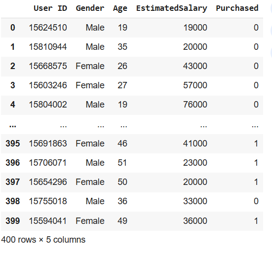
# Load the dataset into a Pandas DataFrame
users = pd.read_csv(dataset_path)
# Display the DataFrame
users
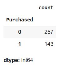
# Count the occurrences of each value in the 'Purchased' column
users.Purchased.value_counts()
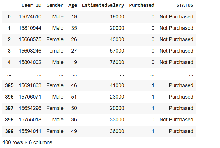
# Add a new column called 'STATUS' based on the 'Purchased' column
users['STATUS'] = users.Purchased.apply(lambda x : 'Not Purchased' if x == 0 else 'Purchased')
# Display the updated DataFrame
users
# Select features (Age and EstimatedSalary) and target (STATUS)
X = users[['Age','EstimatedSalary']] # Features
y = users['STATUS'] # Target
# Display the shapes of features and target
X.shape, y.shape
((400, 2), (400,))
# Display the first few rows of the target variable
y.head()
# Count the occurrences of each value in the 'STATUS' column
users.STATUS.value_counts()
# Split the data into training and testing sets
X_train, X_test, y_train, y_test= train_test_split(X,y, test_size=0.20,random_state=10)
# Display the shapes of training and testing sets
X_train.shape,X_test.shape,y_train.shape,y_test.shape
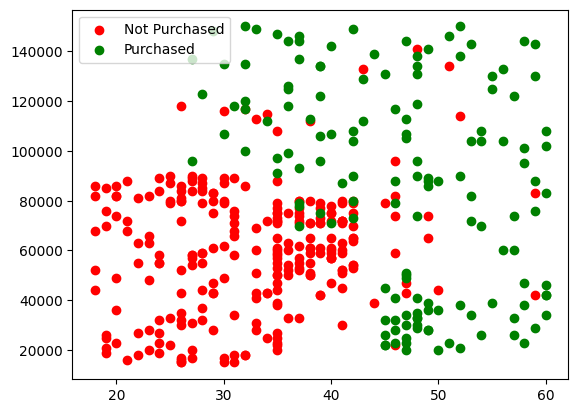
# Plot the data points for 'Not Purchased' and 'Purchased'
plt.scatter(x='Age', y='EstimatedSalary', data=X[y=='Not Purchased'] ,c='red', label='Not Purchased')
plt.scatter(x='Age', y='EstimatedSalary', data=X[y=='Purchased'] ,c='green', label='Purchased')
plt.legend()
plt.show()
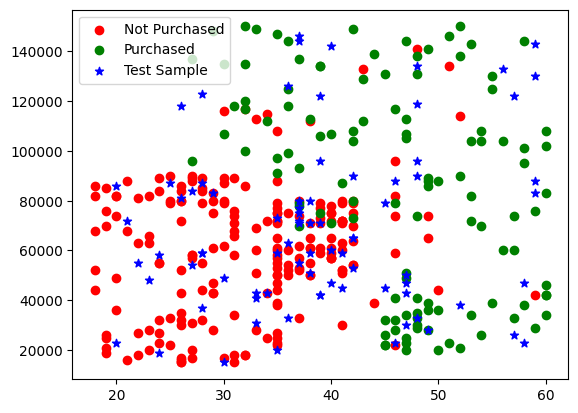
# Plot the training and testing data points
plt.scatter(x='Age', y='EstimatedSalary', data=X_train[y_train == 'Not Purchased'], c='red', label='Not Purchased')
plt.scatter(x='Age', y='EstimatedSalary', data=X_train[y_train == 'Purchased'], c='green', label='Purchased')
plt.scatter(x='Age', y='EstimatedSalary', data=X_test, c='blue', marker='*' ,label='Test Sample')
plt.legend()
plt.show()
# Create and train the Decision Tree model
model = DecisionTreeClassifier(criterion='entropy', max_depth=5)
model.fit(X_train, y_train)
# Make predictions on the test set
y_predict = model.predict(X_test)
# Display the predictions
y_predict
array(['Not Purchased', 'Purchased', 'Not Purchased', 'Purchased',
       'Not Purchased', 'Purchased', 'Not Purchased', 'Purchased',
       'Not Purchased', 'Not Purchased', 'Not Purchased', 'Purchased',
       'Purchased', 'Purchased', 'Purchased', 'Not Purchased',
       'Not Purchased', 'Not Purchased', 'Not Purchased', 'Purchased',
       'Not Purchased', 'Not Purchased', 'Purchased', 'Purchased',
       'Purchased', 'Not Purchased', 'Not Purchased', 'Purchased',
       'Purchased', 'Not Purchased', 'Not Purchased', 'Not Purchased',
       'Not Purchased', 'Purchased', 'Purchased', 'Not Purchased',
       'Purchased', 'Purchased', 'Not Purchased', 'Not Purchased',
       'Not Purchased', 'Purchased', 'Not Purchased', 'Not Purchased',
       'Not Purchased', 'Not Purchased', 'Purchased', 'Not Purchased',
       'Purchased', 'Not Purchased', 'Purchased', 'Purchased',
       'Purchased', 'Not Purchased', 'Not Purchased', 'Purchased',
       'Purchased', 'Not Purchased', 'Purchased', 'Purchased',
       'Not Purchased', 'Purchased', 'Not Purchased', 'Purchased',
       'Purchased', 'Not Purchased', 'Not Purchased', 'Purchased',
       'Not Purchased', 'Not Purchased', 'Purchased', 'Purchased',
       'Not Purchased', 'Not Purchased', 'Not Purchased', 'Not Purchased',
       'Not Purchased', 'Not Purchased', 'Purchased', 'Purchased'],
      dtype=object)
# Display the training target values
y_train
| STATUS | |
|---|---|
| 303 | Purchased |
| 349 | Not Purchased |
| 149 | Not Purchased |
| 100 | Not Purchased |
| 175 | Not Purchased |
| ... | ... |
| 369 | Purchased |
| 320 | Purchased |
| 15 | Not Purchased |
| 125 | Not Purchased |
| 265 | Purchased |
320 rows × 1 columns
dtype: object
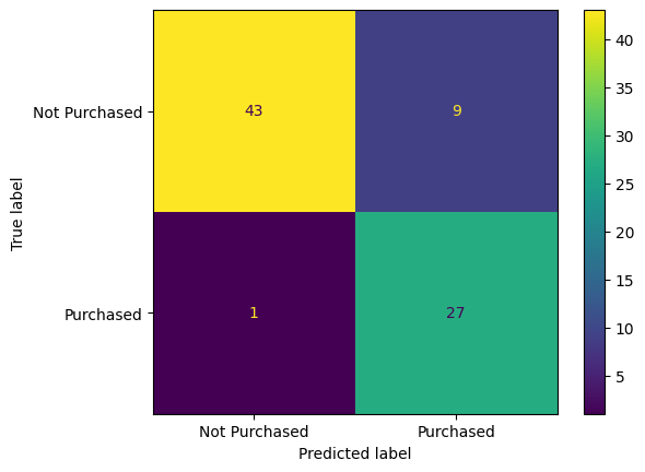
# Calculate and display the accuracy of the model
accuracy = accuracy_score(y_test, y_predict)
accuracy
0.875
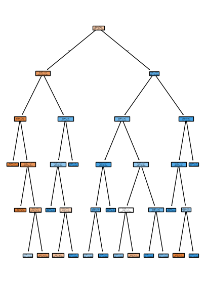
# Visualize the Decision Tree
plt.figure(figsize=(5,7))
plot_tree(model, feature_names=['Age','EstimatedSalary'], class_names=['Not Purchased','Purchased'], filled=True)
plt.show()
# Export the Decision Tree rules as text
tree_rules = export_text(model, feature_names=['Age','EstimatedSalary'], class_names=['Not Purchased', 'Purchased'])
print(tree_rules)


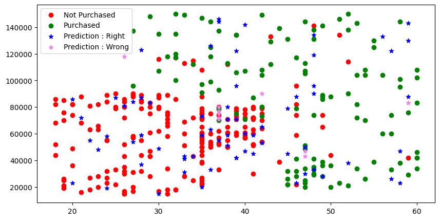
# Plot the data points with predictions and boundaries
plt.figure(figsize=(10,5))
plt.scatter(x='Age', y='EstimatedSalary', data=X_train[y_train=='Not Purchased'], c='red', label='Not Purchased')
plt.scatter(x='Age', y='EstimatedSalary', data=X_train[y_train!='Not Purchased'], c='green', label='Purchased')
plt.scatter(x='Age', y='EstimatedSalary', data=X_test[y_predict==y_test], c='blue', label='Prediction : Right', marker='*')
plt.scatter(x='Age', y='EstimatedSalary', data=X_test[y_predict!=y_test], c='violet', label='Prediction : Wrong', marker='*')
plt.legend()
plt.show()
# Display the confusion matrix
ConfusionMatrixDisplay.from_predictions(y_test, y_predict)
plt.show()
# Display the classification report
classification_report(y_test, y_predict).split('\n')

# Create a DataFrame for new data
data={
'Age' : [30,45],
'EstimatedSalary' : [87000,87000]
}
new_data = pd.DataFrame(data)
# Display the new data
new_data
| Age | EstimatedSalary | |
|---|---|---|
| 0 | 30 | 87000 |
| 1 | 45 | 87000 |
# Make predictions on the new data
prediction = model.predict(new_data)
# Display the predictions
prediction
array(['Not Purchased', 'Purchased'], dtype=object)